Sampling

With pIMF it is possible to draw stochastic samples from the imf.

This tutorial notebook can be downloaded and ran on your own system.

Motivation

Why would you even want to draw individual stars from the IMF?

Scientifically, this is thought to be important when dealing with clusters below \(\sim 10^4\:\mathrm{M}_\odot\). I won’t try to list all codes and papers that are used for fear of omission. But a good starting point might be the third SLUG (Stochastically Lighting Up Galaxies) paper. This is because at a certain total mass, the probability of forming a massive star dips below 0.

We can roughly arrive at this critical mass as follows:

Integrating the IMF from \(M_\star\) to \(M_\textrm{max}\) gives us the probability of forming a star of at least mass \(M_\star\). Setting this to 1 means we are guaranteed to form a star of this mass or greater.

(1)\[\begin{equation} \int_{M_\star}^{M_\textrm{max}}\xi(M)\mathrm{d}M = 1. \end{equation}\]

We can set the normalisation of the IMF by noting the total mass is given by

(2)\[\begin{equation} \int_{M_\textrm{min}}^{M_\textrm{max}}M\xi(M)\mathrm{d}M = M_\textrm{total}. \end{equation}\]

One can calculate the expected maximum mass observed given a total mass or a total mass given an expected maximum mass. In either case, we find that for a Salpeter (1955) with a minimum (maximum) mass \(0.1 (100)\:\mathrm{M}_\odot\):

• to form one star \(90\:\mathrm{M}_\odot\) or greater the total mass must be \(2.6\times 10^4\:\mathrm{M}_\odot\).

• If we form \(5\times10^4\:\mathrm{M}_\odot\) of stars then we will form one star of at least \(95\:\mathrm{M}_\odot\).

These are the limits of what we can consider well-sampled, as otherwise we are accounting for a massive star which might not be formed when we average.

Implementation

In the docstring for draw_samples it says that the imf instance we pass needs to include an inverse_cdf method. This should be a big hint as to how we sample the IMF.

We use inverse CDF sampling (also called inverse transform sampling), which works by generating uniformly random numbers, and plugging them into the inverse of the cumulative distribution function (CDF), also known as the quantile function.

This means any IMF we want to sample needs to have an inverse_cdf method calculated. Luckily we have already calculated CDFs of all our functions in the integrate function, but need to make a change, \(\xi_0 \rightarrow \xi_0 / N\), to make our representation generally the same as a PDF.

Generating Samples

Below we’ll cover how to generate samples with a fixed number of stars, and a fixed mass in stars.

A fixed number of stars

To generate a fixed number of stars, all you need to do is

1. generate random numbers however you want, and

2. plug them into the inverse_CDF method of your IMF of choice.

from pimf import PowerLawIMF

imf = PowerLawIMF(normalisation="number")

import numpy as np
import matplotlib.pyplot as plt

def summarise_sample(masses, plot=True):
    print(f"Generated {len(masses)} stars with a minimum mass of {min(masses):.2f}, a maximum of {max(masses):.1f}, and a total mass of {sum(masses):.2f}.")
    if not plot:
        return
    M = np.geomspace(0.1, 100)

    # Create a histogram of our sample
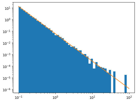
    plt.hist(
        masses,
        density=True,  # Density plots it as a PDF
        bins=M  # space bins evenly in log-space
        )

    # Overplot the IMF
    plt.plot(
        M,
        imf(M)
    )

    plt.xscale("log")
    plt.yscale("log")
    plt.show()

# With python
from random import random

N = 10_000
masses = []

for i in range(N):
    uniform_random_number = random()
    drawn_mass = imf.inverse_cdf(uniform_random_number)
    masses.append(drawn_mass)

summarise_sample(masses)

Generated 10000 stars with a minimum mass of 0.10, a maximum of 76.3, and a total mass of 3694.99.

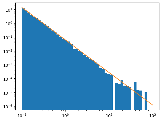
All the included IMFs’ inverse_cdf methods are vectorised, which means you can leverage numpy for faster generation of samples.

rng = np.random.default_rng()
random_numbers = rng.random(size=N)  # Same N as before

masses = imf.inverse_cdf(random_numbers)

summarise_sample(masses)

Generated 10000 stars with a minimum mass of 0.10, a maximum of 65.6, and a total mass of 3521.06.

A fixed mass of stars

In general we don’t know a priori how many stars form, instead having a certain amount of mass.

At its simplest we can just drop an IMF into draw_samples.

from pimf import draw_samples

masses = draw_samples(imf)
summarise_sample(masses)

---------------------------------------------------------------------------
ValueError                                Traceback (most recent call last)
Cell In[4], line 4
      1 from pimf import draw_samples
      2 
      3 masses = draw_samples(imf)
----> 4 summarise_sample(masses)

Cell In[1], line 9, in summarise_sample(masses, plot)
      8 def summarise_sample(masses, plot=True):
----> 9     print(f"Generated {len(masses)} stars with a minimum mass of {min(masses):.2f}, a maximum of {max(masses):.1f}, and a total mass of {sum(masses):.2f}.")
     10     if not plot:
     11         return
     12     M = np.geomspace(0.1, 100)

ValueError: min() iterable argument is empty

By default, we use the mass of the IMF as our target mass, and this IMF has a very small mass.

We can change the imf to have a different normalisation:

imf2 = PowerLawIMF(normalisation="mass", normalisation_value=1000)
masses = draw_samples(imf2)
summarise_sample(masses)

Or, we can use the target_mass argument:

masses = draw_samples(imf, target_mass=1000)
summarise_sample(masses)

How to stop?

If you’re shooting for a target mass, and generating random masses, you won’t end up at your exact target mass.

There are three standard methods for how to choose when to stop. They revolve around the final mass you draw. Call \(M_\textrm{total}^{i-1}\) the total mass before drawing the mass \(m^i\).

1. If \(M_\textrm{total}^{i-1} + m^i > M_\textrm{target}\), discard \(m^i\), so \(M_\textrm{total}^{i-1}\) is the final total mass.

2. Even if \(M_\textrm{total}^{i-1} + m^i > M_\textrm{target}\), keep \(m^i\), so \(M_\textrm{total}^{i-1} + m^i\) is the final total mass.

3. Keep or discard \(m^i\) based on which of \(M_\textrm{total}^{i-1}\) and \(M_\textrm{total}^{i-1}+m^i\) is closer to \(M_\textrm{target}\).

You can switch between them using the stop_method keyword argument to draw_samples, where we call them below, above and closest.

We also have 2 experimental ways of getting results that are closer to the target mass:

1. smith2021_sampling is a function that implemements the sampling method described by Smith (2021). Long story short, when you oversample one IMF you undersample the next, changing the target mass. This should be more accurate in the long run.

2. The rescale argument of draw_samples rescales each mass in the sample by \(M_\mathrm{target}/M_\mathrm{total}\).

Note

The absolute difference between the final total mass and target mass will be at most the upper mass limit of the IMF. For the closest method it is half of the upper mass limit. This means that your relative error will go down with the total mass formed.

for stop_method in ["above", "below", "closest"]:
    print(stop_method, end=": ")
    masses = draw_samples(imf, target_mass=1000, stop_method=stop_method)
    summarise_sample(masses, plot=False)

Seeding Random Numbers

The random numbers aren’t truly random, but depend on some initial condition, called the ‘seed’. Specifing this seed means you will always have the same output, which is useful for reproducing results or trying to fix bugs.

The draw_samples method takes an rng keyword argument, which should be an instance of a numpy Generator. This means you can set the seed as below.

Technically, you can pass anything to rng that has a uniform method with a size argument. However, I have no idea why you want to.

seed = 7
rng = np.random.default_rng(seed=seed)
masses = draw_samples(imf, target_mass=1000, rng=rng)

# Now, reset the random number generator
rng = np.random.default_rng(seed=seed)
masses2 = draw_samples(imf, target_mass=1000, rng=rng)

print(np.all(masses == masses2))

Warning

Check out the numpy docs for their discussion on using big enough seeds. There is a risk that only ever using small seeds (i.e. picking your birthday) will result in regions of state space you never reach, biasing results.

Dealing with Samples

We have a semi-experimental setup for storing and manipulating samples of masses from the IMF, including being able to save to/read from disk.

This is done with the IMFSample and IMFSampleList classes. The former is a list of masses drawn in one realisation. The latter is a way to do operations on a list of IMFSample objects. For example, if you want to study how stochastically sampling the IMF influence the number of ionising photons, you could generate 100 realisations of 1000 solar masses of stars, and compare the total photon output over their lives.