Tutorial
This tutorial notebook can be downloaded and ran on your own system.
from pimf import PowerLawIMF

import numpy as np
import matplotlib.pyplot as plt
Let’s start by looking at the doctring:
help(PowerLawIMF)
Help on class PowerLawIMF in module pimf.initialmassfunction:

class PowerLawIMF(InitialMassFunction)
 |  PowerLawIMF(alpha=-2.35, normalisation='number', normalisation_value=1, Mmin=0.1, Mmax=100)
 |
 |  Implement a power law IMF of the form $\xi(m)dm = \xi_0 m^\alpha dm$.
 |
 |  You can specify if you want to normalise by mass or number, and the range.
 |  If a number is passed to normalisation then it is used
 |  If no normalisation is specified, then we use "number", which with `normalisation_value=1` will yield a PDF.
 |
 |  Normalisation value provides the value we are normalising to, i.e. if you want the IMF to represent 100 solar masses.
 |
 |  With the default slope of -2.35 this represents a Salpeter (1955) IMF.
 |
 |  Method resolution order:
 |      PowerLawIMF
 |      InitialMassFunction
 |      builtins.object
 |
 |  Methods defined here:
 |
 |  __call__(self, M)
 |      Calculate the value $\xi(m) = \xi_0 m^\alpha$.
 |
 |  __init__(self, alpha=-2.35, normalisation='number', normalisation_value=1, Mmin=0.1, Mmax=100)
 |      Initialize self.  See help(type(self)) for accurate signature.
 |
 |  __str__(self)
 |      Return str(self).
 |
 |  integrate(self, Mmin, Mmax)
 |      Gives the analytical solution to the integral:
 |          $\int^{M_{max}}_{M_{min}} \xi(m)dm = \xi_0 \frac{M_{max}^{\alpha+1} - M_{min}^{\alpha+1}}{\alpha + 1}$.
 |
 |      ```{warning}
 |      For performance reasons we do not check Mmin < Mmax, or are within the bounds provided for normalisation.
 |      ```
 |
 |  integrate_product(self, Mmin, Mmax)
 |      Gives the analytical solution to the integral:
 |          $\int^{M_{max}}_{M_{min}} m\xi(m)dm = \xi_0 \frac{M_{max}^{\alpha+2} - M_{min}^{\alpha+2}}{\alpha + 2}$.
 |
 |      ```{warning}
 |      For performance reasons we do not check Mmin < Mmax, or are within the bounds provided for normalisation.
 |      ```
 |
 |  inverse_cdf(self, x)
 |      Calculate the inverse cumulative distribution function for this IMF.
 |
 |      MATHS
 |
 |      This is intended to be used for stochastically sampling stars from the IMF using `LINK`
 |
 |      Parameters
 |      ----------
 |      x : int, float, or numpy array
 |          The value of the CDF at a given mass. Between 0 and 1.
 |
 |      Returns
 |      -------
 |      type of x
 |          The mass(es) that give the x value(s) in the CDF.
 |
 |  ----------------------------------------------------------------------
 |  Methods inherited from InitialMassFunction:
 |
 |  integrate_linear_piecewise_interpolated_product(self, a, b, x, y, extrapolate_grid=False)
 |      Integrate between a and b, assuming the IMF is multiplied by a linear piecewise function defined by the points (xi, yi).
 |
 |      Assume f s.t. f(xi) = yi, where f is linear and piecewise. This function solves the integral $\int^b_a f(m)\xi(m)dm$.
 |
 |      Passing `extrapolate_grid=True` (`False` by default) will use the slope between (x0, y0), (x1, y1) for x < x0, and similarly for x > xN.
 |
 |  mean_mass(self, Mmin, Mmax)
 |      Calculate mean mass of an IMF.
 |
 |      $$M_\mathrm{mean} = \frac{\int^{M_\mathrm{max}}_{M_\mathrm{min}} m\xi(m)\mathrm{d}m}{\int^{M_\mathrm{max}}_{M_\mathrm{min}} m\xi(m)\mathrm{d}m}$$
 |
 |      Parameters
 |      ----------
 |      Mmin : int or float
 |          Minimum mass.
 |      Mmax : int or float.
 |          Maximum mass.
 |
 |      Returns
 |      -------
 |      float
 |          The mean mass of a star for the IMF.
 |
 |  normalise_by_mass(self, Mmin, Mmax, value=1)
 |      Normalise the IMF by mass, so $\int^{M_\mathrm{max}}_{M_\mathrm{min}} m\xi(m)\mathrm{d}m = x$, where x is a user provided value, default 1.
 |
 |  normalise_by_number(self, Mmin, Mmax, value=1)
 |      Normalise the IMF by number, so $\int^{M_\mathrm{max}}_{M_\mathrm{min}} \xi(m)\mathrm{d}m = x$, where x is a user provided value, default 1.
 |
 |  set_normalisation(self, ξ0)
 |      Directly set the normalisation constant $\xi_0$, storing the flag normalised.
 |
 |  ----------------------------------------------------------------------
 |  Data descriptors inherited from InitialMassFunction:
 |
 |  __dict__
 |      dictionary for instance variables
 |
 |  __weakref__
 |      list of weak references to the object
It’s hard to read the unformatted latex (so the readthedocs might be better) but we can see that this class implements an IMF that looks like
Creating an IMF instance
In some cases it’s as simple as:
my_imf = PowerLawIMF()
because we have tried to choose sensible defaults. In other IMFs, there aren’t necessarily sensible defaults. The parameters you are most likely to want to tweak are probably normalisation and normalisation_value, which we explain more below.
Generating Values
All IMFs have a __call__ method, so can be called like functions in python. This just evaluates \(\xi(M)\). You can pass floats or numpy arrays.
print(my_imf(1))
print(my_imf(10))
0.06030765986622325
0.0002693844214326307
# Generate mass values
M = np.geomspace(0.1, 100)
print(my_imf(M))
[1.35012033e+01 9.69381943e+00 6.96013037e+00 4.99735065e+00
 3.58808128e+00 2.57623052e+00 1.84972502e+00 1.32809646e+00
 9.53568878e-01 6.84659309e-01 4.91583126e-01 3.52955063e-01
 2.53420571e-01 1.81955134e-01 1.30643186e-01 9.38013765e-02
 6.73490789e-02 4.83564165e-02 3.47197475e-02 2.49286642e-02
 1.78986987e-02 1.28512066e-02 9.22712394e-03 6.62504455e-03
 4.75676014e-03 3.41533809e-03 2.45220148e-03 1.76067257e-03
 1.26415710e-03 9.07660628e-04 6.51697337e-04 4.67916538e-04
 3.35962531e-04 2.41219989e-04 1.73195156e-04 1.24353551e-04
 8.92854394e-05 6.41066509e-05 4.60283639e-05 3.30482134e-05
 2.37285082e-05 1.70369906e-05 1.22325031e-05 8.78289686e-06
 6.30609098e-06 4.52775252e-06 3.25091137e-06 2.33414364e-06
 1.67590744e-06 1.20329601e-06]
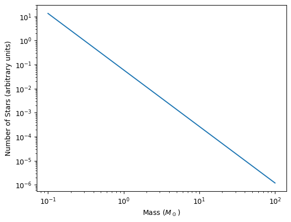
plt.loglog(M, my_imf(M))
plt.xlabel("Mass ($M_\\odot$)")
plt.ylabel("Number of Stars (arbitrary units)")
plt.show()
Integrating
Let’s say we wanted to calculate the number of black holes that form. A simple model might be that any stars below 25 solar masses don’t form a black hole, while stars above this limit do. We could use something like the trapezium rule or a numerical integration routine with the __call__ method. But! We can do better.
For most IMFs it is easy enough to write down an analytic solution to the integral, and that is what we implement in the integrate method.
number_stars_below_25Msol = my_imf.integrate(0.1, 25)
number_stars_above_25Msol = my_imf.integrate(25, 100)
print(f"There are {number_stars_below_25Msol} stars below 25 solar masses, and {number_stars_above_25Msol} above.")
There are 0.9995099448493988 stars below 25 solar masses, and 0.0004900551506009985 above.
At this point, you should be wondering what these values actually mean. After all, you never said how many stars there were in total, or the total stellar mass (which is more common). That is what we will cover in normalisation.
Normalisation
We provide a set of methods for normalising the IMF, but it’s easiest to do it when you initialise the class using the normalise and normalisation_value arguments. When you print an imf, it will tell you how its been normalised.
These fix the value of \(\xi_0\) by calculating the integral, or taking a value from the user.
normalise
There are three options for normalise:
“mass”, a string, requires
normalisation_value“number”, a string, requires
normalisation_valueAny int or float
“mass”
When normalising by mass we rearrange
“number”
When normalising by number we rearrange
Any int or float
If you pass a number as opposed to one of the strings, then it just uses this value for \(\xi_0\).
Let’s say we want to create an IMF that represents 2000 stars, and ask how many black holes that forms.
two_thousand_stars = PowerLawIMF(normalisation="number", normalisation_value=2000)
number_stars_below_25Msol = two_thousand_stars.integrate(0.1, 25)
number_stars_above_25Msol = two_thousand_stars.integrate(25, 100)
print(f"There are {number_stars_below_25Msol} stars below 25 solar masses, and {number_stars_above_25Msol} above.")
There are 1999.0198896987977 stars below 25 solar masses, and 0.9801103012019969 above.
Or, we could ask how many sun-like stars are there in the milky way? Taking a milky way mass of \(\sim6\times10^{10}M_\odot\)
milky_way = PowerLawIMF(normalisation="mass", normalisation_value=6e10)
print(f"There are {milky_way.integrate(0.9, 1.1):g} stars within 10% of the sun's mass.")
There are 2.08698e+09 stars within 10% of the sun's mass.
Be careful, as the IMF represents a probability density, to get an actual number you have to integrate over some mass range.
Winner of the longest method name goes to…
integrate_linear_piecewise_interpolated_product
This is not something that everyone will have to use, but it’s code I wrote so I might as well include it. Essentially what this does is solve annoying problems when you want to know the integral of an arbitrary function
# We take some data from the GENEC grids: https://obswww.unige.ch/Research/evol/tables_grids2011/
# Everything in solar units
grid_masses = np.array([0.8, 0.9, 1.0, 1.1, 1.25, 1.35, 1.5, 1.7, 2.0, 2.5, 3.0, 4.0, 5.0, 7, 9, 12, 15, 20, 25, 32, 40, 60, 85, 120])
grid_luminosities = 10**np.array([-0.58999, -0.35509, -0.13714, 0.06467, 0.29537, 0.459878, 0.673904, 0.913744, 1.208899, 1.596045, 1.898976, 2.365394, 2.712744, 3.220316, 3.584321, 3.977491, 4.266387, 4.614872, 4.86599, 5.125097, 5.343182, 5.703098, 5.980312, 6.231065])

plt.loglog(grid_masses, grid_luminosities, "o")
plt.xlabel("Mass / $M_\\odot$")
plt.ylabel("Luminosity / $L_\\odot$")
plt.show()
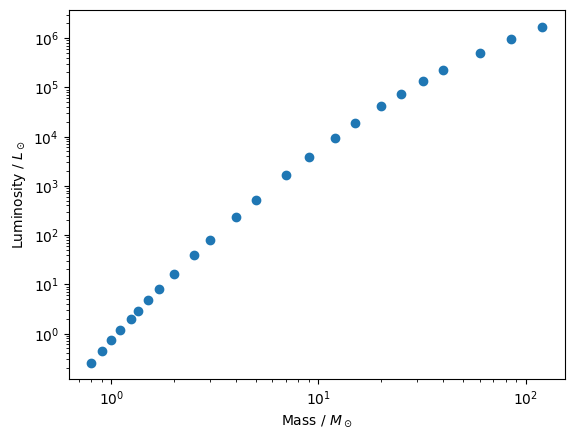
Above we have our grid of mass and luminosity. Let’s use it to answer the question:
Do massive stars contribute more or less to luminosity than low mass stars?
We can see above that luminosity increases increases with mass, but we know that more massive stars are less common. Which effect wins?
# This will return the total luminosity of stars between 0.8 and 8 solar masses, in solar luminosities
low_mass_contribution = my_imf.integrate_linear_piecewise_interpolated_product(
    0.8,               # Minimum mass for integration bounds
    8,                 # Maximum mass for integration bounds
    grid_masses,       # Masses we are interpolating
    grid_luminosities  # Luminosities we are interpolating, the unit of these is our final unit
)

# This will return the total luminosity of stars between 8 and 100 solar masses, in solar luminosities.
high_mass_contribution = my_imf.integrate_linear_piecewise_interpolated_product(
    8,                 # Minimum mass for integration bounds
    100,               # Maximum mass for integration bounds
    grid_masses,       # Masses we are interpolating
    grid_luminosities  # Luminosities we are interpolating, the unit of these is our final unit
)

print(f"{100*low_mass_contribution / (low_mass_contribution + high_mass_contribution) : .2f}% of luminosity comes from low-mass stars")
print(f"{100*high_mass_contribution / (low_mass_contribution + high_mass_contribution) :.2f}% of luminosity comes from high-mass stars")
 2.43% of luminosity comes from low-mass stars
97.57% of luminosity comes from high-mass stars
So massive stars hugely dominate!